This page was generated from pandas3.ipynb.

Exercise 1 (split date continues)	Exercise 2 (cycling weather)	Exercise 3 (top bands)
Exercise 4 (cyclists per day)	Exercise 5 (best record company)	Exercise 6 (suicide fractions)
Exercise 7 (suicide weather)	Exercise 8 (bicycle timeseries)	Exercise 9 (commute)

Pandas (continues)

import pandas as pd
import numpy as np

Catenating datasets

We already saw in the NumPy section how we can catenate arrays along an axis: axis=0 catenates vertically and axis=1 catenates horizontally, and so on. With the DataFrames of Pandas it works similarly except that the row indices and the column names require extra attention. Also note a slight difference in the name: np.concatenate but pd.concat.

Let’s start by considering catenation along the axis 0, that is, vertical catenation. We will first make a helper function to easily create DataFrames for testing.

def makedf(cols, ind):
    data = {c : [str(c) + str(i) for i in ind] for c in cols}
    return pd.DataFrame(data, ind)

Next we will create some example DataFrames:

a=makedf("AB", [0,1])
a

	A	B
0	A0	B0
1	A1	B1

b=makedf("AB", [2,3])
b

	A	B
2	A2	B2
3	A3	B3

c=makedf("CD", [0,1])
c

	C	D
0	C0	D0
1	C1	D1

d=makedf("BC", [2,3])
d

	B	C
2	B2	C2
3	B3	C3

In the following simple case, the concat function works exactly as we expect it would:

pd.concat([a,b])   # The default axis is 0

	A	B
0	A0	B0
1	A1	B1
2	A2	B2
3	A3	B3

The next, however, will create duplicate indices:

r=pd.concat([a,a])
r

	A	B
0	A0	B0
1	A1	B1
0	A0	B0
1	A1	B1

r.loc[0,"A"]

0    A0
0    A0
Name: A, dtype: object

This is not usually what we want! There are three solutions to this. Firstly, deny creation of duplicated indices by giving the verify_integrity parameter to the concat function:

try:
    pd.concat([a,a], verify_integrity=True)
except ValueError as e:
    import sys
    print(e, file=sys.stderr)

Indexes have overlapping values: Int64Index([0, 1], dtype='int64')

Secondly, we can ask for automatic renumbering of rows:

pd.concat([a,a], ignore_index=True)

	A	B
0	A0	B0
1	A1	B1
2	A0	B0
3	A1	B1

Thirdly, we can ask for hierarchical indexing. The indices can contain multiple levels, but on this course we don’t consider hierarchical indices in detail. Hierarchical indices can make a two dimensional array to work like higher dimensional array.

r2=pd.concat([a,a], keys=['first', 'second'])
r2

		A	B
first	0	A0	B0
	1	A1	B1
second	0	A0	B0
	1	A1	B1

r2["A"]["first"][0]

'A0'

Everything works similarly, when we want to catenate horizontally:

pd.concat([a,c], axis=1)

	A	B	C	D
0	A0	B0	C0	D0
1	A1	B1	C1	D1

We have so far assumed that when concatenating vertically the columns of both DataFrames are the same, and when joining horizontally the indices are the same. This is, however, not required:

pd.concat([a,d], sort=False)    # sort option is used to silence a deprecation message

	A	B	C
0	A0	B0	NaN
1	A1	B1	NaN
2	NaN	B2	C2
3	NaN	B3	C3

It expanded the non-existing cases with NaNs. This method is called an outer join, which forms the union of columns in the two DataFrames. The alternative is inner join, which forms the intersection of columns:

pd.concat([a,d], join="inner")

	B
0	B0
1	B1
2	B2
3	B3

---

Exercise 1 (split date continues)

Write function split_date_continues that does

• read the bicycle data set
• clean the data set of columns/rows that contain only missing values
• drops the Päivämäärä column and replaces it with its splitted components as before

Use the concat function to do this. The function should return a DataFrame with 25 columns (first five related to the date and then the rest 20 conserning the measument location.

---

Merging dataframes

Merging combines two DataFrames based on some common field.

Let’s recall the earlier DataFrame about wages and ages of persons:

df = pd.DataFrame([[1000, "Jack", 21], [1500, "John", 29]], columns=["Wage", "Name", "Age"])
df

	Wage	Name	Age
0	1000	Jack	21
1	1500	John	29

Now, create a new DataFrame with the occupations of persons:

df2 = pd.DataFrame({"Name" : ["John", "Jack"], "Occupation": ["Plumber", "Carpenter"]})
df2

	Name	Occupation
0	John	Plumber
1	Jack	Carpenter

The following function call will merge the two DataFrames on their common field, and, importantly, will keep the indices aligned. What this means is that even though the names are listed in different order in the two frames, the merge will still give correct result.

pd.merge(df, df2)

	Wage	Name	Age	Occupation
0	1000	Jack	21	Carpenter
1	1500	John	29	Plumber

This was an example of a simple one-to-one merge, where the keys in the Name columns had 1-to-1 correspondence. Sometimes not all the keys appear in both DataFrames:

df3 = pd.concat([df2, pd.DataFrame({ "Name" : ["James"], "Occupation":["Painter"]})], ignore_index=True)
df3

	Name	Occupation
0	John	Plumber
1	Jack	Carpenter
2	James	Painter

pd.merge(df, df3)                # By default an inner join is computed

	Wage	Name	Age	Occupation
0	1000	Jack	21	Carpenter
1	1500	John	29	Plumber

pd.merge(df, df3, how="outer")   # Outer join

	Wage	Name	Age	Occupation
0	1000.0	Jack	21.0	Carpenter
1	1500.0	John	29.0	Plumber
2	NaN	James	NaN	Painter

Also, many-to-one and many-to-many relationships can occur in merges:

books = pd.DataFrame({"Title" : ["War and Peace", "Good Omens", "Good Omens"] ,
                      "Author" : ["Tolstoi", "Terry Pratchett", "Neil Gaiman"]})
books

	Title	Author
0	War and Peace	Tolstoi
1	Good Omens	Terry Pratchett
2	Good Omens	Neil Gaiman

collections = pd.DataFrame([["Oodi", "War and Peace"],
                           ["Oodi", "Good Omens"],
                           ["Pasila", "Good Omens"],
                           ["Kallio", "War and Peace"]], columns=["Library", "Title"])
collections

	Library	Title
0	Oodi	War and Peace
1	Oodi	Good Omens
2	Pasila	Good Omens
3	Kallio	War and Peace

All combinations with matching keys (Title) are created:

libraries_with_books_by = pd.merge(books, collections)
libraries_with_books_by

	Title	Author	Library
0	War and Peace	Tolstoi	Oodi
1	War and Peace	Tolstoi	Kallio
2	Good Omens	Terry Pratchett	Oodi
3	Good Omens	Terry Pratchett	Pasila
4	Good Omens	Neil Gaiman	Oodi
5	Good Omens	Neil Gaiman	Pasila

---

Exercise 2 (cycling weather)

Merge the processed cycling data set (from the previous exercise) and weather data set along the columns year, month, and day. Note that the names of these columns might be different in the two tables: use the left_on and right_on parameters. Then drop useless columns ‘m’, ‘d’, ‘Time’, and ‘Time zone’.

Write function cycling_weather that reads the data sets and returns the resulting DataFrame.

---

---

Exercise 3 (top bands)

Merge the DataFrames UK top40 and the bands DataFrame that are stored in the src folder. Do all this in the parameterless function top_bands, which should return the merged DataFrame. Use the left_on and right_on parameters to merge. Test your function from the main function.

---

Aggregates and groupings

Let us use again the weather dataset. First, we make the column names a bit more uniform and concise. For example the columns Year, m, and d are not uniformly named.

We can easily change the column names with the rename method of the DataFrame. Note that we cannot directly change the index wh.columns as it is immutable.

wh = pd.read_csv("https://www.cs.helsinki.fi/u/jttoivon/dap/data/fmi/kumpula-weather-2017.csv")

wh3 = wh.rename(columns={"m": "Month", "d": "Day", "Precipitation amount (mm)" : "Precipitation",
                         "Snow depth (cm)" : "Snow", "Air temperature (degC)" : "Temperature"})
wh3.head()

	Year	Month	Day	Time	Time zone	Precipitation	Snow	Temperature
0	2017	1	1	00:00	UTC	-1.0	-1.0	0.6
1	2017	1	2	00:00	UTC	4.4	-1.0	-3.9
2	2017	1	3	00:00	UTC	6.6	7.0	-6.5
3	2017	1	4	00:00	UTC	-1.0	13.0	-12.8
4	2017	1	5	00:00	UTC	-1.0	10.0	-17.8

Pandas has an operation that splits a DataFrame into groups, performs some operation on each of the groups, and then combines the result from each group into a resulting DataFrame. This split-apply-combine functionality is really flexible and powerful operation. In Pandas you start by calling the groupby method, which splits the DataFrame into groups. In the following example the rows that contain measurements from the same month belong to the same group:

groups = wh3.groupby("Month")
groups

<pandas.core.groupby.groupby.DataFrameGroupBy object at 0x7fc59376aba8>

Nothing happened yet, but the groupby object knows how the division into groups is done. This is called a lazy operation. We can query the number of groups in the groupby object:

len(groups)

12

We can iterate through all the groups:

for key, group in groups:
    print(key, len(group))

1 31
2 28
3 31
4 30
5 31
6 30
7 31
8 31
9 30
10 31
11 30
12 31

groups.get_group(2)                 # Group with index two is February

	Year	Month	Day	Time	Time zone	Precipitation	Snow	Temperature
31	2017	2	1	00:00	UTC	1.5	4.0	-0.6
32	2017	2	2	00:00	UTC	0.2	5.0	-0.8
33	2017	2	3	00:00	UTC	-1.0	6.0	-0.2
34	2017	2	4	00:00	UTC	2.7	6.0	0.4
35	2017	2	5	00:00	UTC	-1.0	7.0	-2.5
36	2017	2	6	00:00	UTC	-1.0	7.0	-7.3
37	2017	2	7	00:00	UTC	-1.0	8.0	-12.1
38	2017	2	8	00:00	UTC	-1.0	8.0	-8.8
39	2017	2	9	00:00	UTC	-1.0	8.0	-10.1
40	2017	2	10	00:00	UTC	-1.0	8.0	-8.3
41	2017	2	11	00:00	UTC	-1.0	8.0	-5.4
42	2017	2	12	00:00	UTC	-1.0	8.0	-2.7
43	2017	2	13	00:00	UTC	-1.0	8.0	1.5
44	2017	2	14	00:00	UTC	-1.0	8.0	4.4
45	2017	2	15	00:00	UTC	-1.0	8.0	0.0
46	2017	2	16	00:00	UTC	0.9	8.0	0.5
47	2017	2	17	00:00	UTC	0.2	8.0	1.5
48	2017	2	18	00:00	UTC	1.5	5.0	1.9
49	2017	2	19	00:00	UTC	1.1	5.0	2.2
50	2017	2	20	00:00	UTC	2.8	3.0	0.4
51	2017	2	21	00:00	UTC	-1.0	7.0	-2.5
52	2017	2	22	00:00	UTC	12.2	6.0	-4.6
53	2017	2	23	00:00	UTC	0.3	15.0	-0.7
54	2017	2	24	00:00	UTC	-1.0	13.0	-5.3
55	2017	2	25	00:00	UTC	0.4	13.0	-5.6
56	2017	2	26	00:00	UTC	2.5	12.0	-2.0
57	2017	2	27	00:00	UTC	1.0	14.0	-2.3
58	2017	2	28	00:00	UTC	7.7	13.0	2.1

The groupby object functions a bit like a DataFrame, so some operations which are allowed for DataFrames are also allowed for the groupby object. For example, we can get a subset of columns:

groups["Temperature"]

<pandas.core.groupby.groupby.SeriesGroupBy object at 0x7fc593088f28>

For each DataFrame corresponding to a group the Temperature column was chosen. Still nothing was shown, because we haven’t applied any operation on the groups.

The common methods also include the aggregation methods. Let’s try to apply the mean aggregation:

groups["Temperature"].mean()

Month
1     -2.316129
2     -2.389286
3      0.983871
4      2.676667
5      9.783871
6     13.726667
7     16.035484
8     16.183871
9     11.826667
10     5.454839
11     3.950000
12     1.741935
Name: Temperature, dtype: float64

Now what happened was that after the mean aggregation was performed on each group, the results were automatically combined into a resulting DataFrame. Let’s try some other aggregation:

groups["Precipitation"].sum()

Month
1      26.9
2      21.0
3      29.7
4      26.9
5      -5.9
6      59.3
7      14.2
8      70.1
9      51.2
10    173.5
11    117.2
12    133.6
Name: Precipitation, dtype: float64

Ok, the -1.0 values in the Precipitation field are causing trouble here, let’s convert them to zeros:

wh4 = wh3.copy()
wh4.loc[wh4.Precipitation == -1, "Precipitation"] = 0
wh4.loc[wh4.Snow == -1, "Snow"] = 0
wh4.head()

	Year	Month	Day	Time	Time zone	Precipitation	Snow	Temperature
0	2017	1	1	00:00	UTC	0.0	0.0	0.6
1	2017	1	2	00:00	UTC	4.4	0.0	-3.9
2	2017	1	3	00:00	UTC	6.6	7.0	-6.5
3	2017	1	4	00:00	UTC	0.0	13.0	-12.8
4	2017	1	5	00:00	UTC	0.0	10.0	-17.8

wh4.groupby("Month")["Precipitation"].sum()

Month
1      38.9
2      35.0
3      41.7
4      39.9
5      16.1
6      76.3
7      31.2
8      86.1
9      65.2
10    184.5
11    120.2
12    140.6
Name: Precipitation, dtype: float64

Other ways to operate on groups

The aggregations are not the only possible operations on groups. The other possibilities are filtering, transformation, and application.

In filtering some of the groups can be filtered out.

def myfilter(df):                                     # The filter function must return a boolean value
    return df["Precipitation"].sum() >= 150

wh4.groupby("Month").filter(myfilter)                 # Filter out months with total precipitation less that 150 mm

	Year	Month	Day	Time	Time zone	Precipitation	Snow	Temperature
273	2017	10	1	00:00	UTC	0.0	0.0	9.1
274	2017	10	2	00:00	UTC	6.4	0.0	9.2
275	2017	10	3	00:00	UTC	21.5	0.0	8.3
276	2017	10	4	00:00	UTC	12.7	0.0	11.2
277	2017	10	5	00:00	UTC	0.6	0.0	8.8
278	2017	10	6	00:00	UTC	0.7	0.0	7.7
279	2017	10	7	00:00	UTC	11.7	0.0	8.1
280	2017	10	8	00:00	UTC	14.1	0.0	9.3
281	2017	10	9	00:00	UTC	18.3	0.0	8.6
282	2017	10	10	00:00	UTC	24.2	0.0	8.1
283	2017	10	11	00:00	UTC	1.5	0.0	6.9
284	2017	10	12	00:00	UTC	18.1	0.0	6.0
285	2017	10	13	00:00	UTC	0.0	0.0	7.5
286	2017	10	14	00:00	UTC	5.0	0.0	7.2
287	2017	10	15	00:00	UTC	3.3	0.0	8.3
288	2017	10	16	00:00	UTC	0.0	0.0	10.7
289	2017	10	17	00:00	UTC	1.6	0.0	8.5
290	2017	10	18	00:00	UTC	0.0	0.0	8.3
291	2017	10	19	00:00	UTC	0.9	0.0	4.6
292	2017	10	20	00:00	UTC	0.0	0.0	2.0
293	2017	10	21	00:00	UTC	0.0	0.0	0.2
294	2017	10	22	00:00	UTC	0.0	0.0	0.1
295	2017	10	23	00:00	UTC	0.0	0.0	1.3
296	2017	10	24	00:00	UTC	0.0	0.0	0.8
297	2017	10	25	00:00	UTC	8.5	0.0	2.1
298	2017	10	26	00:00	UTC	12.3	2.0	0.3
299	2017	10	27	00:00	UTC	2.7	7.0	-0.3
300	2017	10	28	00:00	UTC	17.1	4.0	3.3
301	2017	10	29	00:00	UTC	3.3	0.0	2.1
302	2017	10	30	00:00	UTC	0.0	0.0	1.2
303	2017	10	31	00:00	UTC	0.0	0.0	-0.4

In a transformation each group’s DataFrame is manipulated in a way that retains its shape. An example of centering values, so that the deviations from the monthly means are shown:

pd.concat([wh4.iloc[:, 0:3],
           wh4.groupby("Month")[["Precipitation", "Snow", "Temperature"]].transform(lambda x : x - x.mean())],
          axis=1)

	Year	Month	Day	Precipitation	Snow	Temperature
0	2017	1	1	-1.254839	-6.903226	2.916129
1	2017	1	2	3.145161	-6.903226	-1.583871
2	2017	1	3	5.345161	0.096774	-4.183871
3	2017	1	4	-1.254839	6.096774	-10.483871
4	2017	1	5	-1.254839	3.096774	-15.483871
5	2017	1	6	-0.954839	3.096774	-15.483871
6	2017	1	7	4.045161	3.096774	-1.483871
7	2017	1	8	-1.254839	5.096774	1.816129
8	2017	1	9	-0.154839	5.096774	2.816129
9	2017	1	10	-0.954839	2.096774	4.016129
10	2017	1	11	-1.254839	0.096774	0.716129
11	2017	1	12	6.745161	0.096774	-0.483871
12	2017	1	13	-1.154839	6.096774	3.416129
13	2017	1	14	-1.154839	1.096774	3.116129
14	2017	1	15	-1.254839	1.096774	-0.483871
15	2017	1	16	-1.254839	1.096774	-1.883871
16	2017	1	17	-1.054839	1.096774	-1.183871
17	2017	1	18	-0.354839	1.096774	3.416129
18	2017	1	19	-1.254839	-1.903226	3.916129
19	2017	1	20	-0.954839	-1.903226	1.716129
20	2017	1	21	-0.854839	-1.903226	0.516129
21	2017	1	22	-1.054839	-1.903226	3.316129
22	2017	1	23	-1.154839	-0.903226	2.416129
23	2017	1	24	-1.254839	-0.903226	0.116129
24	2017	1	25	-0.654839	-0.903226	-1.483871
25	2017	1	26	-1.254839	-0.903226	4.216129
26	2017	1	27	-1.254839	-2.903226	3.916129
27	2017	1	28	0.545161	-2.903226	3.116129
28	2017	1	29	1.345161	-3.903226	2.916129
29	2017	1	30	4.345161	-1.903226	3.316129
...	...	...	...	...	...	...
335	2017	12	2	0.764516	3.516129	-0.341935
336	2017	12	3	2.664516	-1.483871	3.258065
337	2017	12	4	-4.535484	-1.483871	-0.441935
338	2017	12	5	-3.835484	-1.483871	-1.741935
339	2017	12	6	-4.535484	-1.483871	-2.941935
340	2017	12	7	11.764516	-1.483871	-2.541935
341	2017	12	8	-2.535484	-1.483871	3.458065
342	2017	12	9	-4.335484	-1.483871	2.458065
343	2017	12	10	-4.535484	-1.483871	0.258065
344	2017	12	11	-3.235484	-1.483871	-0.341935
345	2017	12	12	30.464516	-1.483871	-0.141935
346	2017	12	13	-0.335484	3.516129	-0.141935
347	2017	12	14	0.664516	2.516129	-0.141935
348	2017	12	15	5.464516	8.516129	-0.041935
349	2017	12	16	-3.235484	4.516129	0.658065
350	2017	12	17	-4.535484	3.516129	-1.641935
351	2017	12	18	-1.035484	3.516129	0.258065
352	2017	12	19	-4.335484	1.516129	-0.741935
353	2017	12	20	-0.935484	1.516129	0.858065
354	2017	12	21	-4.535484	-1.483871	0.758065
355	2017	12	22	-4.535484	-1.483871	-1.841935
356	2017	12	23	3.064516	-1.483871	-0.541935
357	2017	12	24	-4.535484	-1.483871	-2.041935
358	2017	12	25	1.364516	-1.483871	-1.441935
359	2017	12	26	3.264516	-1.483871	0.158065
360	2017	12	27	-3.435484	-1.483871	2.058065
361	2017	12	28	-0.835484	-1.483871	1.058065
362	2017	12	29	3.264516	-1.483871	2.058065
363	2017	12	30	-0.435484	-1.483871	0.758065
364	2017	12	31	-1.335484	-1.483871	-0.141935

365 rows × 6 columns

The apply method is very generic and only requires that for each group’s DataFrame the given function returns a DataFrame, Series, or a scalar. In the following example, we sort within each group by the temperature:

wh4.groupby("Month").apply(lambda df : df.sort_values("Temperature"))

		Year	Month	Day	Time	Time zone	Precipitation	Snow	Temperature
Month
1	4	2017	1	5	00:00	UTC	0.0	10.0	-17.8
	5	2017	1	6	00:00	UTC	0.3	10.0	-17.8
	3	2017	1	4	00:00	UTC	0.0	13.0	-12.8
	2	2017	1	3	00:00	UTC	6.6	7.0	-6.5
	15	2017	1	16	00:00	UTC	0.0	8.0	-4.2
	1	2017	1	2	00:00	UTC	4.4	0.0	-3.9
	24	2017	1	25	00:00	UTC	0.6	6.0	-3.8
	6	2017	1	7	00:00	UTC	5.3	10.0	-3.8
	16	2017	1	17	00:00	UTC	0.2	8.0	-3.5
	11	2017	1	12	00:00	UTC	8.0	7.0	-2.8
	14	2017	1	15	00:00	UTC	0.0	8.0	-2.8
	23	2017	1	24	00:00	UTC	0.0	6.0	-2.2
	20	2017	1	21	00:00	UTC	0.4	5.0	-1.8
	10	2017	1	11	00:00	UTC	0.0	7.0	-1.6
	19	2017	1	20	00:00	UTC	0.3	5.0	-0.6
	7	2017	1	8	00:00	UTC	0.0	12.0	-0.5
	22	2017	1	23	00:00	UTC	0.1	6.0	0.1
	30	2017	1	31	00:00	UTC	0.0	4.0	0.2
	8	2017	1	9	00:00	UTC	1.1	12.0	0.5
	28	2017	1	29	00:00	UTC	2.6	3.0	0.6
	0	2017	1	1	00:00	UTC	0.0	0.0	0.6
	13	2017	1	14	00:00	UTC	0.1	8.0	0.8
	27	2017	1	28	00:00	UTC	1.8	4.0	0.8
	29	2017	1	30	00:00	UTC	5.6	5.0	1.0
	21	2017	1	22	00:00	UTC	0.2	5.0	1.0
	12	2017	1	13	00:00	UTC	0.1	13.0	1.1
	17	2017	1	18	00:00	UTC	0.9	8.0	1.1
	18	2017	1	19	00:00	UTC	0.0	5.0	1.6
	26	2017	1	27	00:00	UTC	0.0	4.0	1.6
	9	2017	1	10	00:00	UTC	0.3	9.0	1.7
...	...	...	...	...	...	...	...	...	...
12	340	2017	12	7	00:00	UTC	16.3	0.0	-0.8
	357	2017	12	24	00:00	UTC	0.0	0.0	-0.3
	355	2017	12	22	00:00	UTC	0.0	0.0	-0.1
	338	2017	12	5	00:00	UTC	0.7	0.0	0.0
	350	2017	12	17	00:00	UTC	0.0	5.0	0.1
	358	2017	12	25	00:00	UTC	5.9	0.0	0.3
	334	2017	12	1	00:00	UTC	3.4	0.0	0.9
	352	2017	12	19	00:00	UTC	0.2	3.0	1.0
	356	2017	12	23	00:00	UTC	7.6	0.0	1.2
	337	2017	12	4	00:00	UTC	0.0	0.0	1.3
	335	2017	12	2	00:00	UTC	5.3	5.0	1.4
	344	2017	12	11	00:00	UTC	1.3	0.0	1.4
	364	2017	12	31	00:00	UTC	3.2	0.0	1.6
	346	2017	12	13	00:00	UTC	4.2	5.0	1.6
	345	2017	12	12	00:00	UTC	35.0	0.0	1.6
	347	2017	12	14	00:00	UTC	5.2	4.0	1.6
	348	2017	12	15	00:00	UTC	10.0	10.0	1.7
	359	2017	12	26	00:00	UTC	7.8	0.0	1.9
	351	2017	12	18	00:00	UTC	3.5	5.0	2.0
	343	2017	12	10	00:00	UTC	0.0	0.0	2.0
	349	2017	12	16	00:00	UTC	1.3	6.0	2.4
	363	2017	12	30	00:00	UTC	4.1	0.0	2.5
	354	2017	12	21	00:00	UTC	0.0	0.0	2.5
	353	2017	12	20	00:00	UTC	3.6	3.0	2.6
	361	2017	12	28	00:00	UTC	3.7	0.0	2.8
	360	2017	12	27	00:00	UTC	1.1	0.0	3.8
	362	2017	12	29	00:00	UTC	7.8	0.0	3.8
	342	2017	12	9	00:00	UTC	0.2	0.0	4.2
	336	2017	12	3	00:00	UTC	7.2	0.0	5.0
	341	2017	12	8	00:00	UTC	2.0	0.0	5.2

365 rows × 8 columns

---

Exercise 4 (cyclists per day)

This exercise can give two points at maximum!

Part 1.

Read, clean and parse the bicycle data set as before. Group the rows by year, month, and day. Get the sum for each group. Make function cyclists_per_day that does the above. The function should return a DataFrame. Make sure that the columns Hour and Weekday are not included in the returned DataFrame.

Part 2.

In the main function, using the function cyclists_per_day, get the daily counts. The index of the DataFrame now consists of tuples (Year, Month, Day). Then restrict this data to August of year 2017, and plot this data. Don’t forget to call the plt.show function of matplotlib. The x-axis should have ticks from 1 to 31, and there should be a curve to each measuring station. Can you spot the weekends?

---

---

Exercise 5 (best record company)

We use again the UK top 40 data set from the first week of 1964 in the src folder. Here we define “goodness” of a record company (Publisher) based on the sum of the weeks on chart (WoC) of its singles. Return a DataFrame of the singles by the best record company (a subset of rows of the original DataFrame). Do this with function best_record_company.

---

---

Exercise 6 (suicide fractions)

Load the suicide data set from src folder. This data was originally downloaded from Kaggle. Kaggle contains lots of interesting open data sets.

Write function suicide_fractions that loads the data set and returns a Series that has the country as the (row) index and as the column the mean fraction of suicides per population in that country. In other words, the value is the average of suicide fractions. The information about year, sex and age is not used.

---

---

Exercise 7 (suicide weather)

Copy the function suicide fractions from the previous exercise.

Implement function suicide_weather as described below. We use the dataset of average temperature (over years 1961-1990) in different countries from src/List_of_countries_by_average_yearly_temperature.html (https://en.wikipedia.org/wiki/List_of_countries_by_average_yearly_temperature) . You can use the function pd.read_html to get all the tables from a html page. By default pd.read_html does not know which row contains column headers and which column contains row headers. Therefore, you have to give both index_col and header parameters to read_html. Maku sure you use the country as the (row) index for both of the DataFrames. What is the Spearman correlation between these variables? Use the corr method of Series object. Note the the two Series need not be sorted as the indices of the rows (country names) are used to align them.

The return value of the function suicide_weather is a tuple (suicide_rows, temperature_rows, common_rows, spearman_correlation) The output from the main function should be of the following form:

Suicide DataFrame has x rows
Temperature DataFrame has x rows
Common DataFrame has x rows
Spearman correlation: x.x

You might have trouble when trying to convert the temperatures to float. The is because the negative numbers on that html page use a special unicode minus sign, which looks typographically nice, but the float constructor cannot interpret it as a minus sign. You can try out the following example:

s="\u2212" "5"   # unicode minus sign and five
print(s)
try:
    float(s)
except ValueError as e:
    import sys
    print(e, file=sys.stderr)

−5

could not convert string to float: '−5'

But if we explicitly convert unicode minus sign to normal minus sign, it works:

float(s.replace("\u2212", "-"))

-5.0

---

Time series

If a measurement is made at certain points in time, the resulting values with their measurement times is called a time series. In Pandas a Series whose index consists of dates/times is a time series.

Let’s make a copy of the DataFrame that we can mess with:

wh2 = wh3.copy()
wh2.columns

Index(['Year', 'Month', 'Day', 'Time', 'Time zone', 'Precipitation', 'Snow',
       'Temperature'],
      dtype='object')

The column names Year, Month, and Day are now in appropriate form for the to_datetime function. It can convert these fields into a timestamp series, which we will add to the DataFrame.

wh2["Date"] = pd.to_datetime(wh2[["Year", "Month", "Day"]])
wh2.head()

	Year	Month	Day	Time	Time zone	Precipitation	Snow	Temperature	Date
0	2017	1	1	00:00	UTC	-1.0	-1.0	0.6	2017-01-01
1	2017	1	2	00:00	UTC	4.4	-1.0	-3.9	2017-01-02
2	2017	1	3	00:00	UTC	6.6	7.0	-6.5	2017-01-03
3	2017	1	4	00:00	UTC	-1.0	13.0	-12.8	2017-01-04
4	2017	1	5	00:00	UTC	-1.0	10.0	-17.8	2017-01-05

We can now drop the useless fields:

wh2=wh2.drop(columns=["Year", "Month", "Day"])
wh2.head()

	Time	Time zone	Precipitation	Snow	Temperature	Date
0	00:00	UTC	-1.0	-1.0	0.6	2017-01-01
1	00:00	UTC	4.4	-1.0	-3.9	2017-01-02
2	00:00	UTC	6.6	7.0	-6.5	2017-01-03
3	00:00	UTC	-1.0	13.0	-12.8	2017-01-04
4	00:00	UTC	-1.0	10.0	-17.8	2017-01-05

The following method call will set the Date field as the index of the DataFrame.

wh2 = wh2.set_index("Date")
wh2.head()

	Time	Time zone	Precipitation	Snow	Temperature
Date
2017-01-01	00:00	UTC	-1.0	-1.0	0.6
2017-01-02	00:00	UTC	4.4	-1.0	-3.9
2017-01-03	00:00	UTC	6.6	7.0	-6.5
2017-01-04	00:00	UTC	-1.0	13.0	-12.8
2017-01-05	00:00	UTC	-1.0	10.0	-17.8

We can now easily get a set of rows using date slices:

wh2["2017-01-15":"2017-02-03"]

	Time	Time zone	Precipitation	Snow	Temperature
Date
2017-01-15	00:00	UTC	-1.0	8.0	-2.8
2017-01-16	00:00	UTC	-1.0	8.0	-4.2
2017-01-17	00:00	UTC	0.2	8.0	-3.5
2017-01-18	00:00	UTC	0.9	8.0	1.1
2017-01-19	00:00	UTC	-1.0	5.0	1.6
2017-01-20	00:00	UTC	0.3	5.0	-0.6
2017-01-21	00:00	UTC	0.4	5.0	-1.8
2017-01-22	00:00	UTC	0.2	5.0	1.0
2017-01-23	00:00	UTC	0.1	6.0	0.1
2017-01-24	00:00	UTC	-1.0	6.0	-2.2
2017-01-25	00:00	UTC	0.6	6.0	-3.8
2017-01-26	00:00	UTC	-1.0	6.0	1.9
2017-01-27	00:00	UTC	-1.0	4.0	1.6
2017-01-28	00:00	UTC	1.8	4.0	0.8
2017-01-29	00:00	UTC	2.6	3.0	0.6
2017-01-30	00:00	UTC	5.6	5.0	1.0
2017-01-31	00:00	UTC	-1.0	4.0	0.2
2017-02-01	00:00	UTC	1.5	4.0	-0.6
2017-02-02	00:00	UTC	0.2	5.0	-0.8
2017-02-03	00:00	UTC	-1.0	6.0	-0.2

By using the date_range function even more complicated sets can be formed. The following gets all the Mondays of July:

r=pd.date_range("2017-07-01", "2017-07-31", freq="w-mon")
r

DatetimeIndex(['2017-07-03', '2017-07-10', '2017-07-17', '2017-07-24',
               '2017-07-31'],
              dtype='datetime64[ns]', freq='W-MON')

wh2.index.difference(r)

DatetimeIndex(['2017-01-01', '2017-01-02', '2017-01-03', '2017-01-04',
               '2017-01-05', '2017-01-06', '2017-01-07', '2017-01-08',
               '2017-01-09', '2017-01-10',
               ...
               '2017-12-22', '2017-12-23', '2017-12-24', '2017-12-25',
               '2017-12-26', '2017-12-27', '2017-12-28', '2017-12-29',
               '2017-12-30', '2017-12-31'],
              dtype='datetime64[ns]', length=360, freq=None)

wh2.loc[r,:]

	Time	Time zone	Precipitation	Snow	Temperature
2017-07-03	00:00	UTC	2.2	-1.0	14.5
2017-07-10	00:00	UTC	-1.0	-1.0	18.0
2017-07-17	00:00	UTC	2.7	-1.0	15.4
2017-07-24	00:00	UTC	-1.0	-1.0	15.7
2017-07-31	00:00	UTC	0.1	-1.0	17.8

The following finds all the business days (Monday to Friday) of July:

pd.date_range("2017-07-01", "2017-07-31", freq="b")

DatetimeIndex(['2017-07-03', '2017-07-04', '2017-07-05', '2017-07-06',
               '2017-07-07', '2017-07-10', '2017-07-11', '2017-07-12',
               '2017-07-13', '2017-07-14', '2017-07-17', '2017-07-18',
               '2017-07-19', '2017-07-20', '2017-07-21', '2017-07-24',
               '2017-07-25', '2017-07-26', '2017-07-27', '2017-07-28',
               '2017-07-31'],
              dtype='datetime64[ns]', freq='B')

We can get a general idea about the Temperature column by plotting it. Note how the index time series is shown nicely on the x-axis.

%matplotlib inline
wh2["Temperature"].plot();

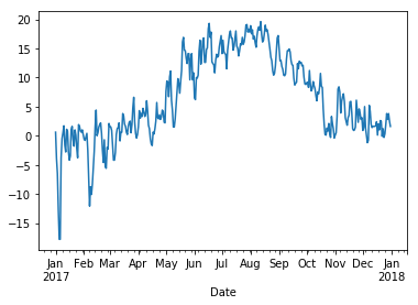
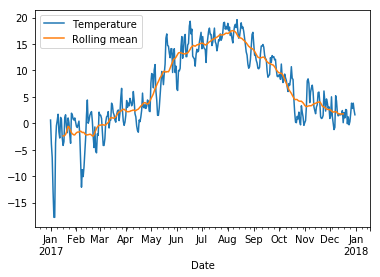
The graph looks a bit messy at this level of detail. We can smooth it by taking averages over a sliding window of length 30 days:

rolling = wh2.Temperature.rolling(30, center=True)
rolling

Rolling [window=30,center=True,axis=0]

data = pd.DataFrame({"Temperature" : wh2.Temperature, "Rolling mean" : rolling.mean()})
data.plot();

---

Exercise 8 (bicycle timeseries)

Write function bicycle_timeseries that

• reads the data set
• cleans it
• turns its Päivämäärä column into (row) DatetimeIndex (that is, to row names) of that DataFrame
• returns the new DataFrame

---

---

Exercise 9 (commute)

In function commute do the following:

Use the function bicycle_timeseries to get the bicycle data. Restrict to August 2017, group by the weekday, aggregate by summing. Set the Weekday column to numbers from one to seven. Then set the column Weekday as the (row) index. Return the resulting DataFrame from the function.

In the main function plot the DataFrame. Xticklabels should be the weekdays. Don’t forget to call show function!

If you want the xticklabels to be ['Mon', 'Tue', 'Wed', 'Thu', 'Fr', 'Sat', 'Sun'] instead of numbers (1,..,7), then it may get a bit messy. There seems to be a problem with non-numeric x values. You could try the following after plotting, but you don’t have to:

weekdays="x mon tue wed thu fri sat sun".title().split()
plt.gca().set_xticklabels(weekdays)

---

Additional information

Pandas cheat sheet Summary of most important Pandas’ functions and methods.

Read the article Tidy Data. The article uses the statistical software R as an example, but the ideas are relevant in general. Pandas operations maintain data in the tidy format.

Pandas handles only one dimensional data (Series) and two dimensional data (DataFrame). While you can use hierarchical indices to simulate higher dimensional arrays, you should use the xarray library, if you need proper higher-dimensional arrays with labels. It is basically a cross between NumPy and Pandas.